Fan Engineering
Thermal Design
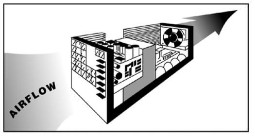
The need for forced-air cooling should be determined at an early stage in system design. It is important that the design plans for good airflow to heat-generating components and also allows adequate space and power for the cooling fan. The first stage in designing a forced-air cooling system is to estimate the required airflow. This depends on the heat generated within the enclosure and the maximum temperature rise permitted.
The airflow required can be obtained either by calculation or from a graph. The equation for calculation is:
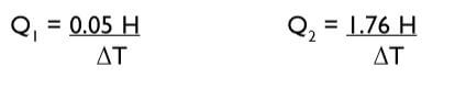
Q1 = Airflow required in m3/min
Q2 = Airflow required in cubic feet/min
H = Heat dissipated in watts
ΔT = Temperature rise above inlet temp °C
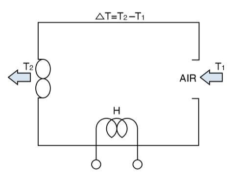
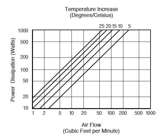
In the following graph, the vertical axis represents the heat to be removed and the horizontal axis represents the airflow; both axes are logarithmic. The sloping lines define the temperature rise in ˚C. To use the graph, find the sloping line that represents the permitted temperature rise. Then, find the point on this line that corresponds to the heat to be removed. The horizontal position of this point shows the airflow required.
System Impedance and Operating Point
Obstructions in the airflow path cause static pressure within the enclosure. To achieve maximum airflow, obstructions should be minimized. However, obstructions in the form of baffles may be necessary to direct the airflow over the components that need cooling.
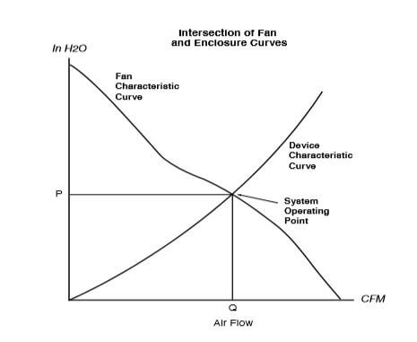
Chart 2.1 illustrates the nonlinear relationship between airflow and static pressure for a typical fan. The System Impedance curve, Chart 2.2, is a property inherent to an individual electronics enclosure. This curve can easily be generated experimentally, by testing the enclosure pressure at various airflow rates. The performance of a fan in a specific application is determined by the intersection of the System Impedance curve and the Fan Characteristic Curve, as shown on Chart 2.3.
Chart 2.1: Typical relationship between Airflow and Static pressure for an Axial cooling fan.
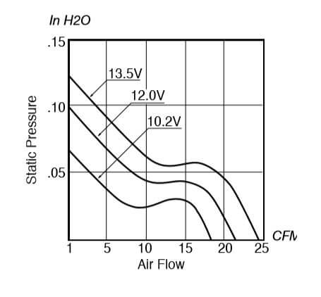
Chart 2.2
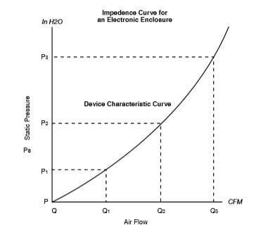
Chart 2.3
Multiple Fan Use
The following figures show the performance characteristics for parallel and series operation of two identical fans.
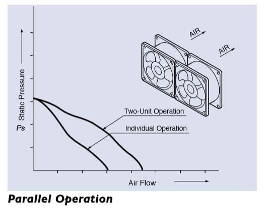
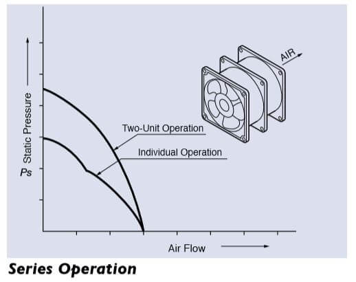
An additional fan in parallel to the first increases airflow in a low static pressure situation. An additional fan in series increases the airflow in a high static- pressure enclosure.
Airflow and Pressure Measurement
An AMCA Standard 210 double chamber is used to accurately measure air volume and static pressure.
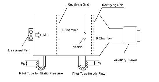
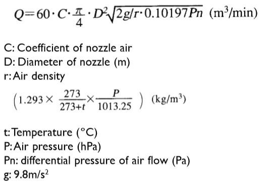
Maximum Static Pressure: When the nozzle is closed, the pressure in chamber A will reach maximum. Maximum Airflow: When opening the nozzle and absorbing the air using the auxiliary blower to make the static pressure zero (Ps = 0), the differential pressure (Pn) between A chamber and B chamber will reach maximum. The airflow obtained by applying the differential pressure (Pn) to the above equation can be called the maximum airflow.
Note: Fan performance is calculated using the data obtained from this equipment according to the following formula:
The Equation: Airflow
Acoustic Noise Measurement
Noise measurements are performed in an Anechoic Chamber with less than 16 dBA background noise in compliance with JIS C 9603 standards. DC Fan 1 m from inlet side AC Fan 1 m from the side.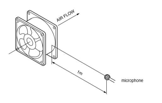
Fan Sensors
Three types of DC fan sensors are available for NMB fans:
- Locked Rotor Signal – outputs the status of the fan motor and is ideal for detecting if the fan motor is rotating or stopped.
- Tachometer Signal – set to produce two cycles of rectangular waveform as the fan motor makes one rotation and is ideal for detecting speed.
- Life Signal – detects a reduction in fan speed at a specified RPM level.
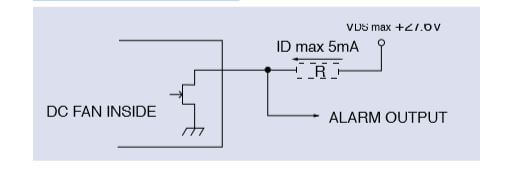
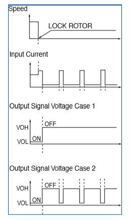
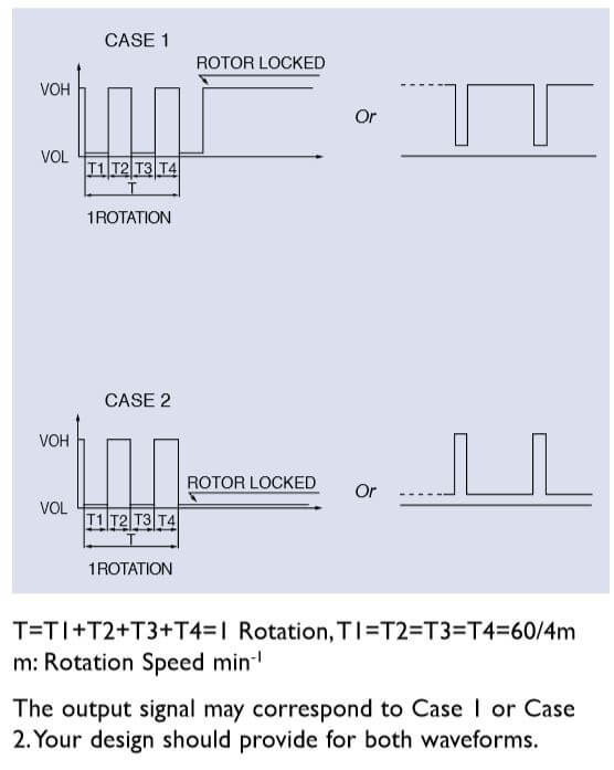
Locked Rotor Alarm Signal:
Output Circuit: Open Collector Specifications: Vce max: +30V Vce max: +15V(1004KL, 1404KL, 1204KL, 1604KL, 1606KL, 1608KL, 2004KL, 2106KL, 2406KL, BM4515, BM5115, BM5125, BM6015)
Ic max: 5mA (Vce(sat)max=0.4V)
Alarm Signal Circuit
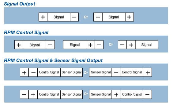
Output Waveform: At rated voltage, the output signal may correspond to either Case 1 or Case 2. Your design should provide for both waveforms.
Tachometer Signal:
Output Waveform: At Rated Voltage
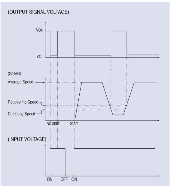
Life Signal:
Output Waveform: At Rated Voltage
Speed Control
DC fan speed can be controlled in order to optimize cooling, reduce noise and decrease system power draw. There are various methods of controlling fan speed.
2-speed DC fan motor
NMB’s custom 2 speed fans are available with high and low speeds specified by the customer. The low end operating speed is fixed in order to reduce noise and lower power consumption.
Below is an example of an External connection for a 2-speed DC fan motor.
Control by relay contact
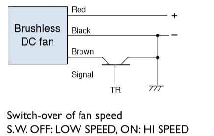
Control by transistor
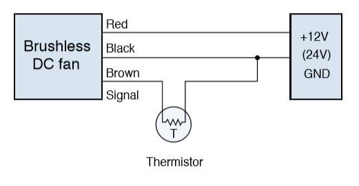
Temperature Detecting Variable Speed DC Fan
The RPM may be automatically controlled and synchronized with temperature variation by installing a thermistor.
Varying the control voltage (0 to 6V) enables speed variation between the signal wire and ground. Example of connection diagram:
PWM Control DC Fan
In PWM speed control, a fixed frequency square wave is applied to the speed control leadwire of the fan.
The ratio of on time vs. off time (duty cycle) is directly proportional to the speed of the fan.
Example:
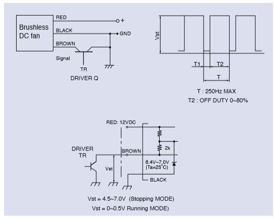
Correct signal connection is important to prevent damage to the internal fan IC. Connection should be design as shown below:
Fan Laws
There are various laws useful in determining different fan performance parameters. We have selected a few of these that can be useful in calculating airflow (CFM), pressure (inches H20), power consumption (Watts), and noise (dBA), when operating at differing speeds (RPM).
Only fans of the same physical dimensions, same motor and impeller should be used for comparative analysis.
The variables below are used in the formulas that follow:
Speed_k = Known Speed
Speed_n = The new speed we are using for calculation
Airflow_k = Known airflow at Speed_k
Airflow_n = New airflow calculated at new speed
Pressure_k = Known Pressure at Speed_k
Pressure_n = New pressure calculated at new speed
Power_k = Known Power at Speed_k
Power_n = New Power calculated at new speed
Noise_k = Known Noise at Speed_k
Noise_n = New Noise calculated at new speed
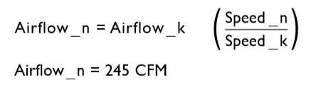
Calculating Airflow at Different Speeds
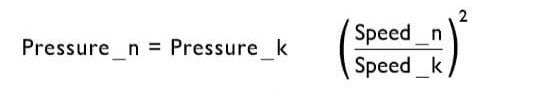
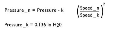
Calculating Pressure at Different Speeds
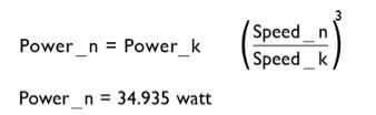
Calculating Power Draw at Different Speeds

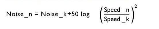
Calculating Noise at Different Speeds
Airflow Calculation Example:
If a fan provides 210 CFM of airflow at 3000 RPM. What airflow (CFM) would be expected if the speed (RPM) is increased to 3500 RPM?
Speed_k = 3000
RPM Airflow k = 210 FM
Speed_n = 3500 RPM
Pressure Calculation Example:
In the example above the fan provides 0.1 inches of H20 Pressure at the system operating point. What pressure would be expected if the fan speed were increased to 3500 RPM?
Speed_k = 3000 RPM
Speed_n = 3500 RPM
Pressure_k = 0.1 in H20
Power Calculation Example:
The fan in question draws 22 Watts at 3000 RPM. What power draw would be expected if the fan speed were increased to 3500 RPM?
Speed_k = 3000 RPM
Speed_n = 3500 RPM
Power_k = 22 watt
Noise Calculation Example:
The fan in question generates 58 dBA of noise measured 1 meter from the inlet side of the fan. What would the increase in noise be if the the speed were increased form 3000 RPM to 3500 RPM?
Speed _ k = 3000 RPM
Speed _ n = 3500 RPM
Noise _ k = 58 dBA

Fan Life and Reliability
Fan Life Testing
Life expectancy of a cooling fan is a critical element in thermal design. NMB uses parametric failure modes during life testing to calculate for life expectancy. Speed (RPM) and Current (mA) failures include both “hard failures” (where the fan is non-functional) and “parametric failures”. These parametric failures are defined as 15% decrease in RPM and an increase in mA of 15%.
Including parametric failure modes leads to a more conservative L-10 and MTTF reporting standard than those methods that measure life performance using only hard failures.
The benefit to the customer is a fan that sets the quality and reliability standard for the cooling industry.
NMB evaluates fan life and reliability during the design phase using accelerated life testing in conjunction with ORT (Ongoing Reliability Testing). Accelerated life testing is used to compress the amount of time required to conduct life testing. Development testing occurs early in the product design, prior to product release. It is vital to characterize the reliability of the product in the initial stages of design to allow for improvements and to meet the reliability specifications prior to release to manufacturing.
Once the design has been through design verification testing and is turned over to manufacturing, ORT is conducted. For some models, ORT evaluation has continued beyond 10 years. The value of ORT is a continued refinement of the accuracy of the accelerated life testing and constant review of the design of the fan. This continued process improvement allows for ongoing evaluation and increase in fan life and reliability.
Under accelerated life testing NMB fans are tested at extreme environmental conditions, with temperature stress factors above standard operating levels. In order to gather meaningful data within a reasonable time frame, the stress factors must be accelerated to simulate different operating environments. High temperature stress is the most common stress factor used for these purposes.
Proper understanding of accelerating stresses and design limits are necessary to implement a meaningful accelerated reliability test. NMB uses the Arrhenius model for determining acceleration factors (AF) during life testing. This is the most commonly used model in accelerated life testing where thermal stress is the primary factor affecting life.
Life test data gathered from different types of fans and blowers lends to highly accurate statistical analysis. This data can produce very detailed information about the behavior of the product for reliability and prediction of fan performance in the field. The Weibull Distribution is a typical method employed by NMB for statistical analysis. An explanation of this calculation model is shown below.
Arrhenius Weibull Model:
Life Stress Relation: Arrhenius
The Arrhenius life-stress relationship is given by:
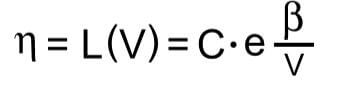
- L represents a quantifiable life measure, which is the scale parameter or characteristic life of the Weibull Distribution.
- V represents the stress level (formulated for temperature and temperature values in absolute units, i.e. degrees Kelvin or degrees Rankine)
- C is one of the model parameters to be determined ( C > 0 ).
- B is another model parameter to be determined
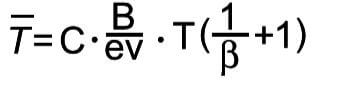
Mean Life or MTTF
The mean, T, also called MTTF or Mean Time To Failure, of the Arrhenius-Weibull relationship is given by:
Reliable Life
The Arrhenius Weibull Distribution model predicts the length of time at which a defined percentage of a product population will still be operating without failing to meet pre-set criteria. For cooling fans, this is normally characterized as L10 life expectancy, or the time at which 10% of a population will have failed and 90% of a population will continue to operate within specifications.
For the Arrhenius-Weibull relationship, the reliable life, TR, of a unit for a specified reliability and starting the mission at age zero is given by:
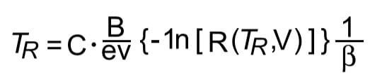
This is the life for which the unit will function successfully with a reliability of R(TR). If R (TR) = 0.90 then TR = 90% reliability or 10% unreliability (L10) or the life by which 90% of the units will survive.
NMB uses parametric failure modes, or the condition at which a performance parameter fails to meet pre-set criteria, to record failures during accelerated life testing. This produces a more accurate prediction of field reliability than methods which use only non-operating failure modes to record failures.
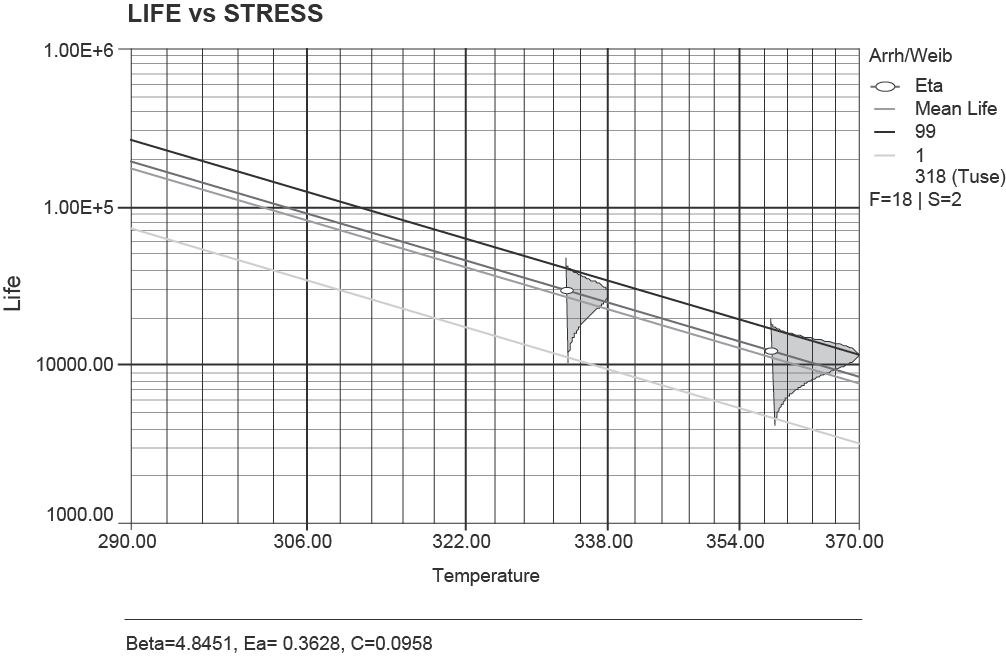
Example: Life Experiment Data Using Arrhenius Weibull
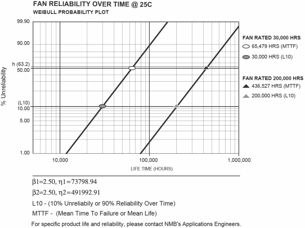
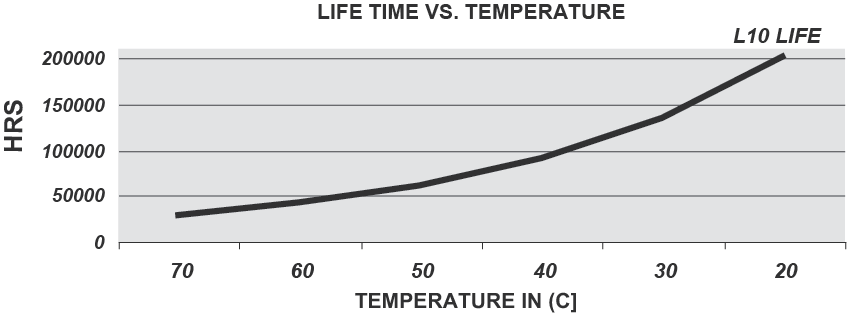
Product L10 life expectancy for NMB fans ranges from 30,000 hours to 200,000 hours of continuous operation at room temperature depending on fan speed, frame size, design structure, size of ball bearings and the type of ball bearings used. NMB, a world leader in miniature precision ball bearings design and manufacturing, uses high quality, long life bearings produced in house to ensure extended fan life.